User’s manual#
The current version of IOSACal is in beta state (i.e. suitable for experimental production use), but has already all the basic functionality, like calibration, generation of publication-quality plots and determination of probability intervals.
What is calibration?#
IOSACal takes a radiocarbon determination and outputs a calibrated age as a set of probability intervals. A radiocarbon date is represented by a date in years BP (before present, that is before 1950 AD) and a standard deviation, like 2430±170. The combination of these two values is a numerical representation of a laboratory measure performed on the original organic material.
The main task of the calibration process is to convert this measure into a set of calendar dates by means of a calibration curve. Users can choose whether they want results as a plot, a short textual summary or both (the plot includes the summary).
IOSACal reads calibration curves in the common .14c format used also by
other programs. Should you have calibration data in another format, it would be
easy to either convert them to that format or modify the source code of IOSACal
to adapt it to your needs.
IOSACal is based on current calibration methods, like those described in [RAM2008].
C. Bronk Ramsey, Radiocarbon dating: revolutions in understanding, Archaeometry 50,2 (2008) pp. 249–275 http://dx.doi.org/10.1111/j.1475-4754.2008.00394.x
Basic usage#
The command line program is called iosacal. It can generate both
text output and image plots.
The typical usage is:
$ iosacal -d 7505 -s 93 --id "P-769"
Output will look like the following:
# P-769

Calibration of P-769: 7505 ± 93 BP

## Calibrated age

Atmospheric data from Reimer et al (2020)

### 68.2% probability

* 8386 CalBP - 8283 CalBP (42.1%)
* 8266 CalBP - 8199 CalBP (26.0%)

### 95.4% probability

* 8515 CalBP - 8500 CalBP (0.8%)
* 8457 CalBP - 8163 CalBP (89.7%)
* 8137 CalBP - 8116 CalBP (1.0%)
* 8102 CalBP - 8039 CalBP (3.9%)
All options can be expressed in short and long versions. The previous command can also be written as:
$ iosacal --date 7505 --sigma --93 --id "P-769"
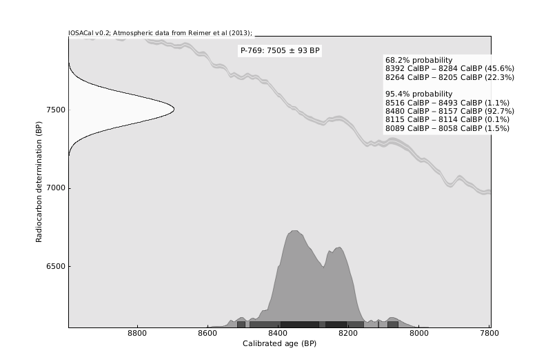
If you want an image instead of text output, just add the -p flag (or the long equivalent --plot):
$ iosacal -d 7505 -s 93 --id "P-769" -p
The result will be saved into the image file named
P-769_7505_93.pdf in the same directory. It will look more or less
like this:
Other calibration curves#
By default, iosacal uses the IntCal20 calibration curve. IOSACal
is however able to read any calibration curve that uses the same
format, such as those available from <http://www.intcal.org/>. If you want to specify a different
calibration curve provide the canonical name of the curve in lower case
(e.g. intcal09, marine09).
To specify a calibration curve, use the -c command line option:
$ iosacal -d 7505 -s 93 --id "P-769" -p -c intcal04
Please note that IOSACal already includes the calibration curves listed below:
IntCal20
Marine20
ShCal20
IntCal13
Marine13
ShCal13
IntCal09
Marine09
IntCal04
Marine04
ShCal04
IntCal98
Marine98
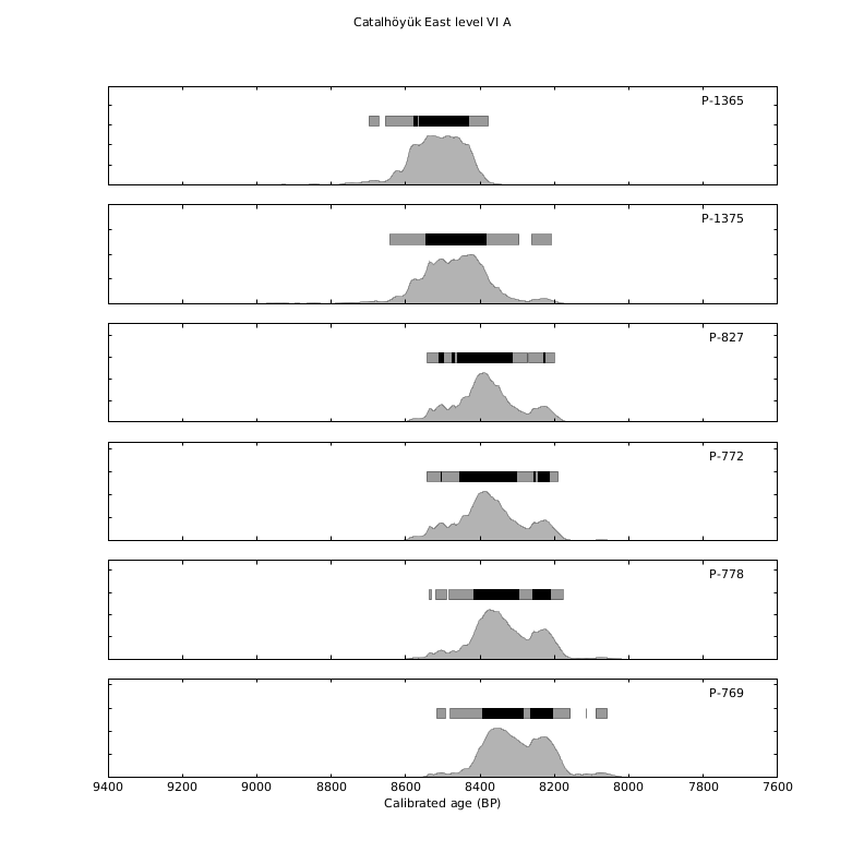
Multiple dates#
It is also possible to give IOSACal more than one radiocarbon determination, to see how 2 or more samples relate between themselves.
To use the multiple dates feature, just pass multiple -d, -s and
--id options on the command line:
$ iosacal \
  -d 7729 -s 80 --id "P-1365" \
  -d 7661 -s 99 --id "P-1375" \
  -d 7579 -s 86 --id "P-827" \
  -d 7572 -s 92 --id "P-772" \
  -d 7538 -s 89 --id "P-778" \
  -d 7505 -s 93 --id "P-769" \
  -p -m -n "Catalhöyük East level VI A"
The order in which values are passed to IOSACal matters, so the first date will be matched to the first standard deviation and so on.
This way, you will get 6 different single plots. The -m flag is used to
indicate you want a compound plot. It’s also useful to use the -n option
to give a name to the image and a title to the plot.
The resulting compound plot looks like this:
Warning
Currently IOSACal doesn’t perform any Bayesian matching of calibrated ages. This feature will be added in future versions.
Command line options#
IOSACal works from the command line. These are the available options.
- --help#
Show an help message and exit
- -d <date>, --date=<date>#
Conventional radiocarbon age, i.e. the non-calibrated radiocarbon BP date for the sample [required]
- -s <sigma>, --sigma=<sigma>#
Error at 1 standard deviation for the non-calibrated date given with the
--dateoption, must be a positive number [required]
- --id <sample_id>#
Lab ID of the sample, e.g. P-1244, OxA-3311 or BETA-248559, but can be any string like “test” if needed [required]
- -c <curve>, --curve=<curve>#
Calibration curve to be used [default:
intcal13]If you want to specify a different calibration curve provide the curve canonical name in lower case (e.g.
intcal09,marine13), or the full path to a file, like/home/user/mycalibrationcurve.14c
Plot output#
- -p, --plot#
Enables the graphical plot output.
- -o, --oxcal#
Plots will be more similar to OxCal [default: False]
- -n <name>, --name <name>#
Specify a name for the output plot [default: “iosacal”]
- -1, --single#
Generate single plots for each sample. The default action.
- --no-single#
Don’t generate single plots for each sample.
- -m, --stacked#
Generate a stacked plot with all samples.
BP or calendar dates#
Use these mutually exclusive options to choose which type of dates you like as output.
- --bp#
Express date in Calibrated BP Age (default action)
- --ad#
Express date in Calibrated BC/AD calendar Age
- --ce#
Express date in Calibrated BCE/CE calendar Age